Scott’s Data Science Blog - Play the audio for the old US ringtone

1 Introduction

The Bell telphone ringtone was a two second tone composed of the frequencies 440 Hz and 480 Hz. The tone was followed by a four second pause, and then repeated. This ringtone continues to be used in the US with most mobile/landline carriers, and PBX systems. Read more about this, and other international ringtones, at https://en.wikipedia.org/wiki/Ringing_tone.

You can download a recording of the US ringtone, which is now in the public domain. Shown below is a demonstration of how to play this sound file within a Jupyter notebook.

from IPython.display import display, HTML, Audio
HTML("""<p>Ringtone Recording:</p>
        <audio controls>
        <source type="audio/mp3"
          src="resources/US_ringback_tone.mp3">
        <source type="audio/ogg"
          src="resources/US_ringback_tone.ogg">
        <p>Your browser cannot play this audio</p>
        </audio>""")

Ringtone Recording:

2 Basics of audio frequencies

Let’s start with some basics before jumping into recreating this ringtone.

The sounds that we hear are produced by longitudinal pressure waves in air particles. These waves cause your ear drum to vibrate. A pure tone is produced when you hear an unchanging frequency with a sinusoidal waveform.

The basic equation of a sinusoidal waveform:

\(y(t) = sin \left({ 2 \pi f t }\right)\)

Where, \(t\) is the time value, and \(f\) = wave frequency (Hertz).

2.1 Symbolic equations in Python

If you are exploring a problem it can be helpful to start with symbolic computation. The Sympy package in Python allows you to operate on and simplify algebraic equations. Then, when you are ready, you can easily convert your equations into numerical formats (e.q., a Python list, or a Numpy array).

Define sinusoidal waveform equation as a symbolic equation.

import sympy as s

# Define variables as Sympy symbols
t, f = s.symbols('t f')

# Define Sympy equation
y = s.sin(2*s.pi*t*f)

print(f"y = {y}")

y = sin(2*pi*f*t)

2.2 Musical notes

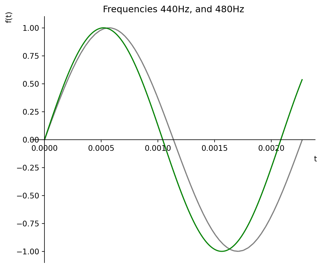
As a first example let’s explore a couple of pure tones: 440 Hz (A4), and 480 Hz (B4).

# Substitue these frequencies in for f
y_at_440_hz = y.subs(f, 440)
y_at_480_hz = y.subs(f, 480)

# Show the new equations
print(f"y_at_440_hz = {y_at_440_hz}")
print(f"y_at_480_hz = {y_at_480_hz}")

y_at_440_hz = sin(880*pi*t)
y_at_480_hz = sin(960*pi*t)

2.3 Plot the notes A4 and B4 on a graph

Let’s plot these example frequencies together on a graph. Note that we don’t have to transform our equations into numerical lists before plotting them. Sympy does this for us. We just need to provide a plot range.

plot_range = (t, 0, 1/440)

# Plot the curve for A4
p = s.plot(
    y_at_440_hz, plot_range, 
    line_color='gray',
    title=f'Frequencies 440Hz, and 480Hz',
    show=False)

# Add the curve for B4 to the graph
p.extend(s.plot(
    y_at_480_hz, plot_range, 
    line_color='green',
    show=False, adaptive=False))

# Format the graph and display it
p.size = (6,5)
p.show()

2.4 Convert Sympy equations into Python lists

In order to listen to these two notes we need to convert the equations into numerical time series.

# Convert our Sympy equations into 
# Python lambda functions
lambda_y_440 = s.lambdify(t, y_at_440_hz)
lambda_y_480 = s.lambdify(t, y_at_480_hz)

# Define numeric values for f1, and f2
f_440, f_480 = (440, 480)
# Number of samples per cycle
n = 50
# Number of seconds of play time
play_time = 3
# Sampling period in micro-seconds
t_440_delta = int(1e6/n/f_440)
t_480_delta = int(1e6/n/f_480) 
# Total play time in micro-seconds
t_max = int(play_time*1e6)

# Iterators for each time series
ts_440_range = range(0, t_max, t_440_delta)
ts_480_range = range(0, t_max, t_480_delta)

# Generate numeric lists from lambda
# functions.  Note: time (t) values have 
# to be converted back into seconds.
ts_440 = [lambda_y_440(t/1e6) 
          for t 
          in ts_440_range]
ts_480 = [lambda_y_480(t/1e6) 
           for t 
           in ts_480_range]

2.5 Play sounds for A4 and B4

Audio(ts_440, rate=f_440*n)

Audio(ts_480, rate=f_480*n)

3 Recreate the US ringtone

In the United States, the ringtone has historically been a two second tone composed of the frequencies 440 Hz and 480 Hz. The tone is followed by a four second pause, and then repeated until the call is answered.

3.1 Acoustic Equations

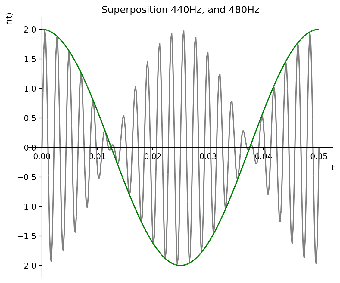
When multiple sound waves overlap, their amplitudes add together. This is called superposition.

\(y_{super}(t) = sin \left({ 2 \pi f_1 t }\right) + sin \left({ 2 \pi f_2 t }\right)\)

Where, the beat frequency (\(f_{beat}\)) is defined as

\(f_{beat} = \lvert f_1 - f_2 \rvert\),

and the beat waveform equation (\(y_{beat}\)) is defined as

\(y_{beat}(t) = 2 \cdot cos \left({ 2 \pi f_{beat} t }\right)\)

# Define variables as Sympy symbols
t, f = s.symbols('t f')

# Define Sympy equations
y = s.sin(2*s.pi*t*f)
y_beat = 2*s.cos(s.pi*t*f)

# Define the two numeric frequencies
f1 = 440
f2 = 480
# Calculate beat frequency
f_beat = abs(f1-f2)

# Substitute in the numeric values
y_super = y.subs(f, f1) + y.subs(f, f2)
y_beat = y_beat.subs(f, f_beat)

# Display the simplified equations
print(f"y_super = {y_super}")
print(f"y_beat = {y_beat}")

y_super = sin(880*pi*t) + sin(960*pi*t)
y_beat = 2*cos(40*pi*t)

3.2 Plot the superpositioned waveforms on a graph

Plot the superpositioned frequencies along with the curve for the beat frequency.

plot_range = (t, 0, 2/f_beat)

# Plot the superpositioned waveform in gray
p = s.plot(
    y_super, plot_range, line_color='gray',
    title=f'Superposition {f1}Hz, and {f2}Hz',
    show=False, adaptive=False)

# Plot, on the same graph, the beat frequency 
# function in green.
p.extend(
    s.plot(y_beat, plot_range, 
           line_color='green', 
           show=False, adaptive=False))
p.size = (6,5)
p.show()

3.3 Convert Sympy equations to numeric lists

# Convert our Sympy equation into a
# Python lambda function
lambda_y_ringtone = s.lambdify(t, y_super)

# Number of samples per cycle
n = 50
# Number of seconds of play time
play_time = 2
# Sampling period in micro-seconds
t_delta = int(1e6/n/max(f1,f2))
# Total play time in micro-seconds
t_max = int(play_time*1e6)

# Create the time series as a list
ts_ringtone = [
   lambda_y_ringtone(t/1e6) 
   for t 
   in range(0,t_max, t_delta)]

pause_4sec = [
    0.0
    for t 
    in range(0,2*t_max,t_delta)]

3.4 Play the ringtone sound

audio_sampling_rate = max(f1,f2)*n

print('audio_sampling_rate =', 
      audio_sampling_rate, 'Hz')

audio_sampling_rate = 24000 Hz

Audio(ts_ringtone + pause_4sec + ts_ringtone, 
      rate=audio_sampling_rate)